Getting started with moultmcmc • moultmcmc

To install moultmcmc please follow the instructions in the README file.

library(moult)
library(moultmcmc)
library(dplyr)
library(ggplot2)
library(rstan)

For demonstration purposes we use the sanderlings dataset from Underhill and Zucchini (1988). It contains observations of sampling dates Day and moult indices MIndex for 164 adult Sanderlings (Calidris alba) trapped on 11 days in the South Africa in the austral summer of 1978/79. The sample contains 85 pre-moult individuals, 66 in active moult and 13 post-moult individuals. The data are augmented with a column describing categorical moult status MCat, so we can demonstrate fitting Type 1 models when data are coded categorically.

data("sanderlings")
sanderlings$MCat <- case_when(sanderlings$MIndex == 0 ~ 1,
                              sanderlings$MIndex == 1 ~3,
                              TRUE ~ 2)
#plot the data
ggplot(sanderlings, aes(y=MIndex, x=Day, col = factor(MCat))) + geom_point() +theme_classic()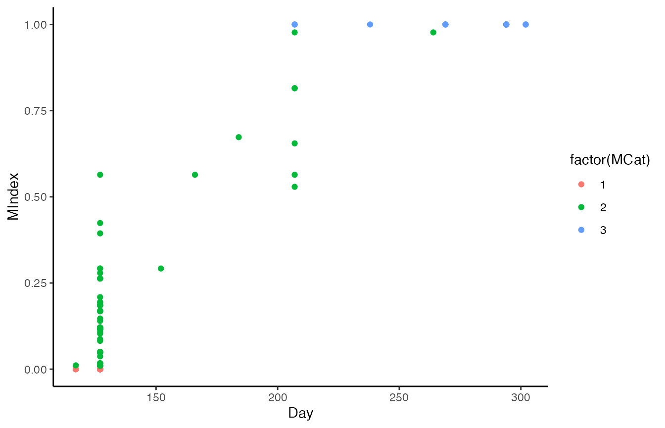

The central function for model fitting is the moultmcmc() function. Model variants of the standard Underhill-Zucchini models are specified using the type argument to designate the relevant input data type. Additionally the user has to designate the input data columns containing moult records, and dates, respectively, as well as linear predictor structures for the main moult parameters - the start date, duration and the standard deviation of the start date. To fit an intercept-only type 1 model we therefore use the following specification:

mcmc1 = moultmcmc(moult_column = "MCat",
                  date_column = "Day",
                  start_formula = ~1,
                  duration_formula = ~1,
                  sigma_formula = ~1,
                  data = sanderlings,
                  type=1,
                  init = "auto",
                  chains = 2,
                  refresh=1000)
#> 
#> SAMPLING FOR MODEL 'uz1_linpred' NOW (CHAIN 1).
#> Chain 1: 
#> Chain 1: Gradient evaluation took 0.000155 seconds
#> Chain 1: 1000 transitions using 10 leapfrog steps per transition would take 1.55 seconds.
#> Chain 1: Adjust your expectations accordingly!
#> Chain 1: 
#> Chain 1: 
#> Chain 1: Iteration:    1 / 2000 [  0%]  (Warmup)
#> Chain 1: Iteration: 1000 / 2000 [ 50%]  (Warmup)
#> Chain 1: Iteration: 1001 / 2000 [ 50%]  (Sampling)
#> Chain 1: Iteration: 2000 / 2000 [100%]  (Sampling)
#> Chain 1: 
#> Chain 1:  Elapsed Time: 0.942 seconds (Warm-up)
#> Chain 1:                0.449 seconds (Sampling)
#> Chain 1:                1.391 seconds (Total)
#> Chain 1: 
#> 
#> SAMPLING FOR MODEL 'uz1_linpred' NOW (CHAIN 2).
#> Chain 2: 
#> Chain 2: Gradient evaluation took 7.6e-05 seconds
#> Chain 2: 1000 transitions using 10 leapfrog steps per transition would take 0.76 seconds.
#> Chain 2: Adjust your expectations accordingly!
#> Chain 2: 
#> Chain 2: 
#> Chain 2: Iteration:    1 / 2000 [  0%]  (Warmup)
#> Chain 2: Iteration: 1000 / 2000 [ 50%]  (Warmup)
#> Chain 2: Iteration: 1001 / 2000 [ 50%]  (Sampling)
#> Chain 2: Iteration: 2000 / 2000 [100%]  (Sampling)
#> Chain 2: 
#> Chain 2:  Elapsed Time: 0.744 seconds (Warm-up)
#> Chain 2:                0.453 seconds (Sampling)
#> Chain 2:                1.197 seconds (Total)
#> Chain 2:

Most MCMC parameters, such as the number of chains (here 2), iterations, or cores are set in the same way as for rstan::sampling, however, for initial values moultmcmc defaults to an additional option "auto" which will provide initial values for the MCMC chains based on the input data. Custom initial values can be specified instead as detailed in the documentation of rstan::sampling.

Once the MCMC has completed, a summary table of parameter estimates can be displayed with

summary_table(mcmc1)
#> # A tibble: 5 × 11
#>   parame…¹ estim…² se_mean     sd     lci     uci n_eff  Rhat  prob method type 
#>   <chr>      <dbl>   <dbl>  <dbl>   <dbl>   <dbl> <dbl> <dbl> <dbl> <chr>  <chr>
#> 1 mean_(I…  134.   0.116    3.48   128.    142.    898.  1.00  0.95 MCMC   1    
#> 2 duratio…   97.6  0.314   10.6     78.1   119.   1144.  1.00  0.95 MCMC   1    
#> 3 log_sd_…    3.34 0.00671  0.228    2.89    3.78 1155.  1.00  0.95 MCMC   1    
#> 4 sd_(Int…   28.9  0.196    6.60    18.0    43.8  1131.  1.00  0.95 MCMC   1    
#> 5 lp__     -104.   0.0418   1.21  -107.   -103.    840.  1.00  0.95 MCMC   1    
#> # … with abbreviated variable names ¹parameter, ²estimate

and standard model assessment can be done as for any posterior sample from Stan, by directly accessing the stanfit slot of the returned S3 object. For example we can look at the traceplots for the model using rstan::stan_trace

stan_trace(mcmc1$stanfit)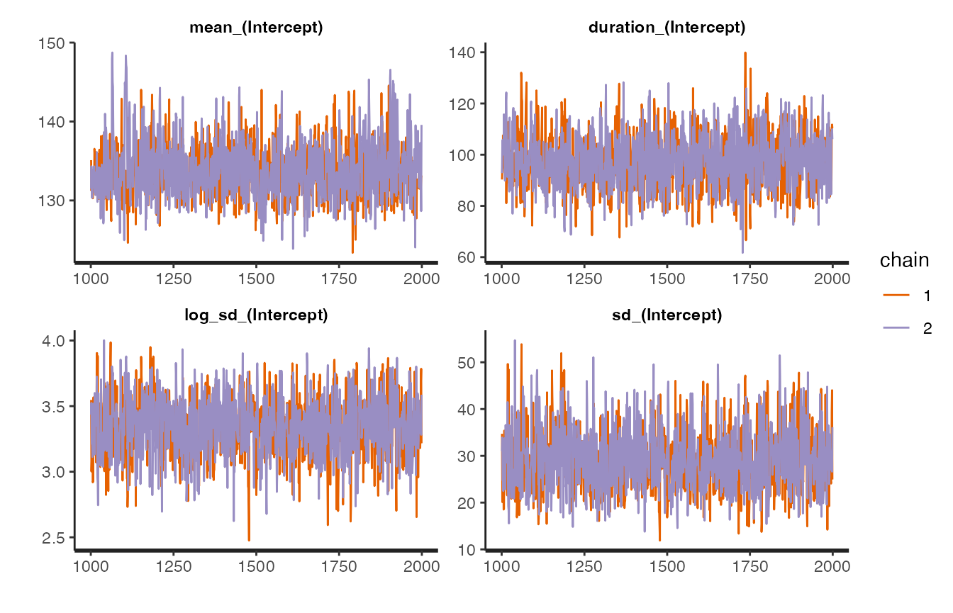

We can also plot the model fit against the data using the moult_plot function

moult_plot(mcmc1)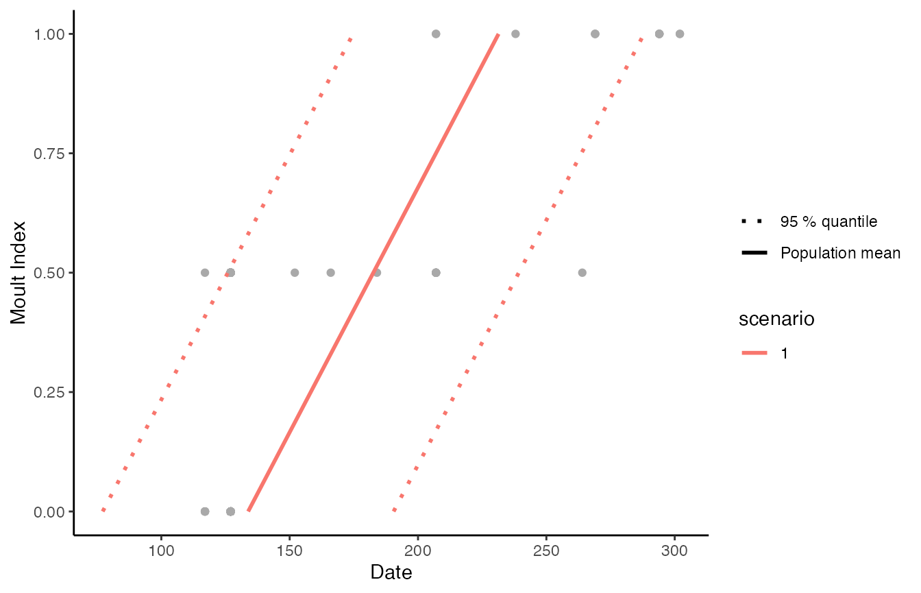

For comparison we can fit the same model using maximum likelihood estimation via the moult package (Erni et al. 2013) and compare parameter estimates visually with the compare_plot function.

ml1 = moult(MIndex ~ Day,data = sanderlings, type = 1)
compare_plot(ml1, mcmc1)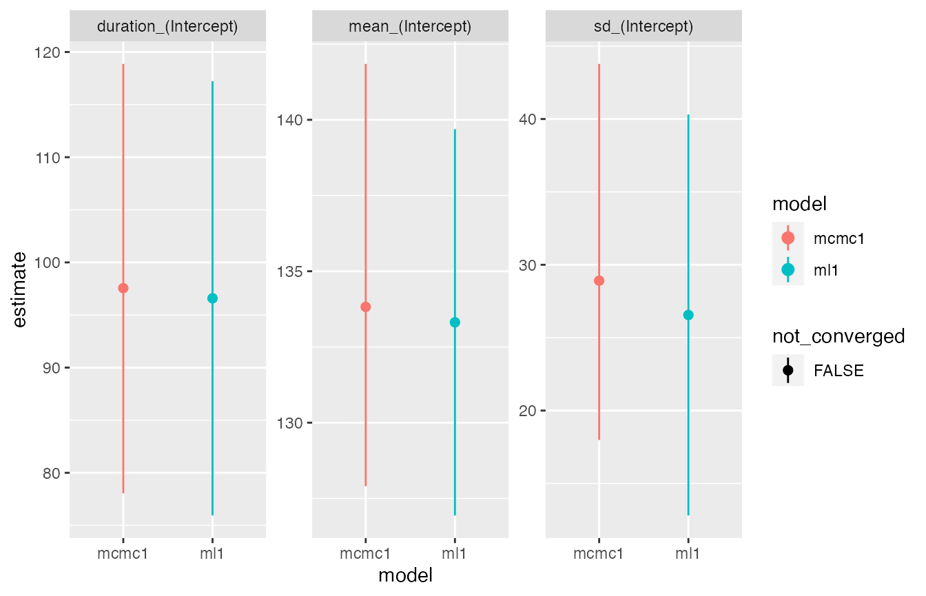

The comparison plot shows very similar estimates for both methods.

Similarly we can fit the corresponding Type 2 model, that makes use of the full information contained in the moult indices, by setting type=2. All moultmcmc models default to an intercept only model, so we do not need to explicitly specify the individual linear predictors here.

#fit using MCMC
mcmc2 = moultmcmc(moult_column = "MIndex",
                date_column = "Day",
                type=2,
                data = sanderlings,
                chains = 2,
                refresh = 1000)
#> 
#> SAMPLING FOR MODEL 'uz2_linpred' NOW (CHAIN 1).
#> Chain 1: 
#> Chain 1: Gradient evaluation took 7.4e-05 seconds
#> Chain 1: 1000 transitions using 10 leapfrog steps per transition would take 0.74 seconds.
#> Chain 1: Adjust your expectations accordingly!
#> Chain 1: 
#> Chain 1: 
#> Chain 1: Iteration:    1 / 2000 [  0%]  (Warmup)
#> Chain 1: Iteration: 1000 / 2000 [ 50%]  (Warmup)
#> Chain 1: Iteration: 1001 / 2000 [ 50%]  (Sampling)
#> Chain 1: Iteration: 2000 / 2000 [100%]  (Sampling)
#> Chain 1: 
#> Chain 1:  Elapsed Time: 0.75 seconds (Warm-up)
#> Chain 1:                0.366 seconds (Sampling)
#> Chain 1:                1.116 seconds (Total)
#> Chain 1: 
#> 
#> SAMPLING FOR MODEL 'uz2_linpred' NOW (CHAIN 2).
#> Chain 2: 
#> Chain 2: Gradient evaluation took 4.3e-05 seconds
#> Chain 2: 1000 transitions using 10 leapfrog steps per transition would take 0.43 seconds.
#> Chain 2: Adjust your expectations accordingly!
#> Chain 2: 
#> Chain 2: 
#> Chain 2: Iteration:    1 / 2000 [  0%]  (Warmup)
#> Chain 2: Iteration: 1000 / 2000 [ 50%]  (Warmup)
#> Chain 2: Iteration: 1001 / 2000 [ 50%]  (Sampling)
#> Chain 2: Iteration: 2000 / 2000 [100%]  (Sampling)
#> Chain 2: 
#> Chain 2:  Elapsed Time: 0.689 seconds (Warm-up)
#> Chain 2:                0.267 seconds (Sampling)
#> Chain 2:                0.956 seconds (Total)
#> Chain 2:
#fit using ML
ml2 = moult(MIndex ~ Day,data = sanderlings, type = 2)
#compare parameter estimates
compare_plot(ml2, mcmc2)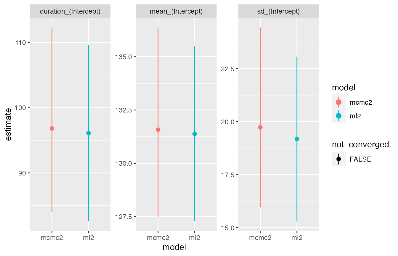

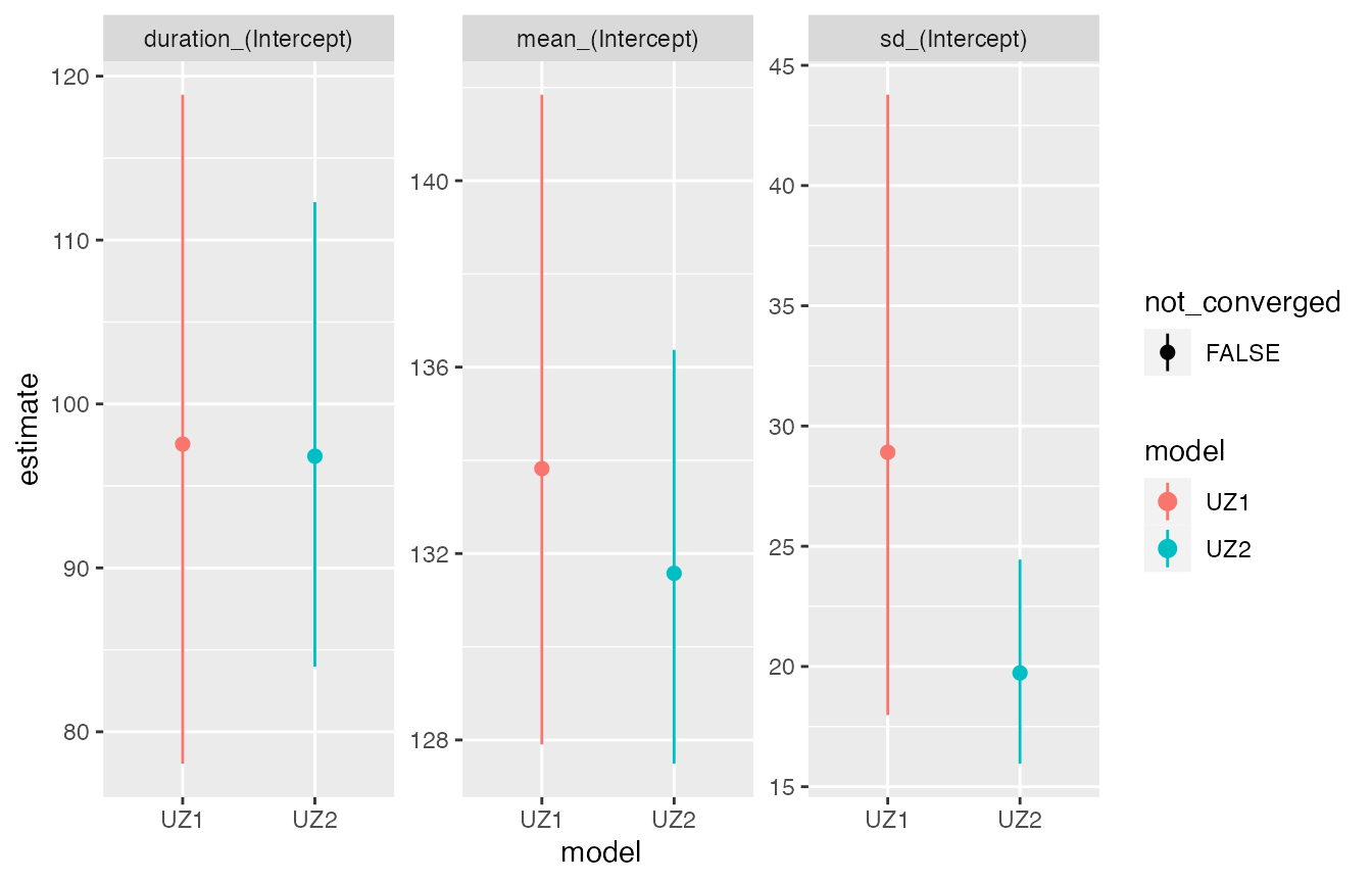
As before the comparison plot shows very similar estimates for both methods. Perhaps more interesting is a comparison of the two model types, which illustrates the gain in precision achieved by exploiting the information contained in the moult indices. Note that models can be given custom names for visualisation purposes using the names argument to compare_plot

compare_plot(mcmc1, mcmc2, names = c('UZ1','UZ2'))

References

Erni, Birgit, Bo T. Bonnevie, Hans-Dieter Oschadleus, Res Altwegg, and Les G. Underhill. 2013. “Moult: An R Package to Analyze Moult in Birds.” Journal of Statistical Software 52. https://doi.org/10.18637/jss.v052.i08.

Underhill, Les G., and Walter Zucchini. 1988. “A Model for Avian Primary Moult.” Ibis 130: 358–72. https://doi.org/10.1111/j.1474-919x.1988.tb00993.x.