Extended moult models
extended-moult-models.RmdTo install moultmcmc please follow the instructions in
the README
file.
Lumped models
The gradual transition from new to old plumage between successive
moults can make the assignment of non-moulting birds to pre-moult and
post-moult categories ambiguous. This classification problem can be
sidestepped by distinguishing only two categories of birds: moulting and
non-moulting birds, which is implemented in the so called “lumped” moult
models in moultmcmc.
The following example demonstrates the use of the lumped type 2 moult
model. It is based on a dataset originally supplied with the
moult package (Erni et al.
2013) on Southern Masked Weavers (Ploceus velatus), all
caught in the Western Cape province of South Africa (Oschadleus 2005). For convenience the data set
is provided with processed moult scores in moultmcmc as
weavers_processed.
data(weavers_processed)
weavers_processed <- filter(weavers_processed, Year %in% 1993:2003)
ggplot(weavers_processed, aes(x=day, y =pfmg)) +
  geom_point() + theme_classic() +
  ylab('PFMG') + xlab('Days since 01 August')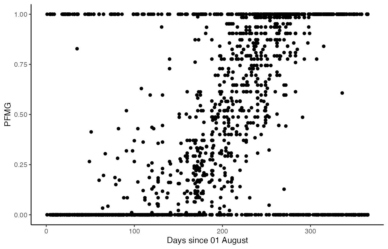
We then fit both standard and lumped type 2 moult models to this
dataset. The lumped model can be activated by setting the option
lump_non_moult = TRUE.
mc2 <- moultmcmc('pfmg',
                 'day',
                 data=weavers_processed,
                 chains = 2, cores = 2)
mc2l <- moultmcmc('pfmg',
                  'day',
                  data=weavers_processed,
                  lump_non_moult = TRUE,
                  chains = 2, cores = 2)
We also fit a type 3 model to these data, following the recommendation in Erni et al. (2013). This model type only uses active moult records, and therefore is unaffected by misclassification in the non-moulting birds.
mc3 <- moultmcmc('pfmg',
                 'day',
                 data=weavers_processed,
                 type = 3,
                 chains = 2, cores=2)
cowplot::plot_grid(
   moult_plot(mc2) + theme(legend.position='none') +
     xlim(-150,575) + ggtitle('Type 2 model'),
   moult_plot(mc2l) + theme(legend.position='none') +
     xlim(-150,575) + ggtitle('Lumped type 2 model (T2L)'),
   moult_plot(mc3) + theme(legend.position='bottom') +
     xlim(-150,575) + ggtitle('Type 3 model'),
   nrow=3
)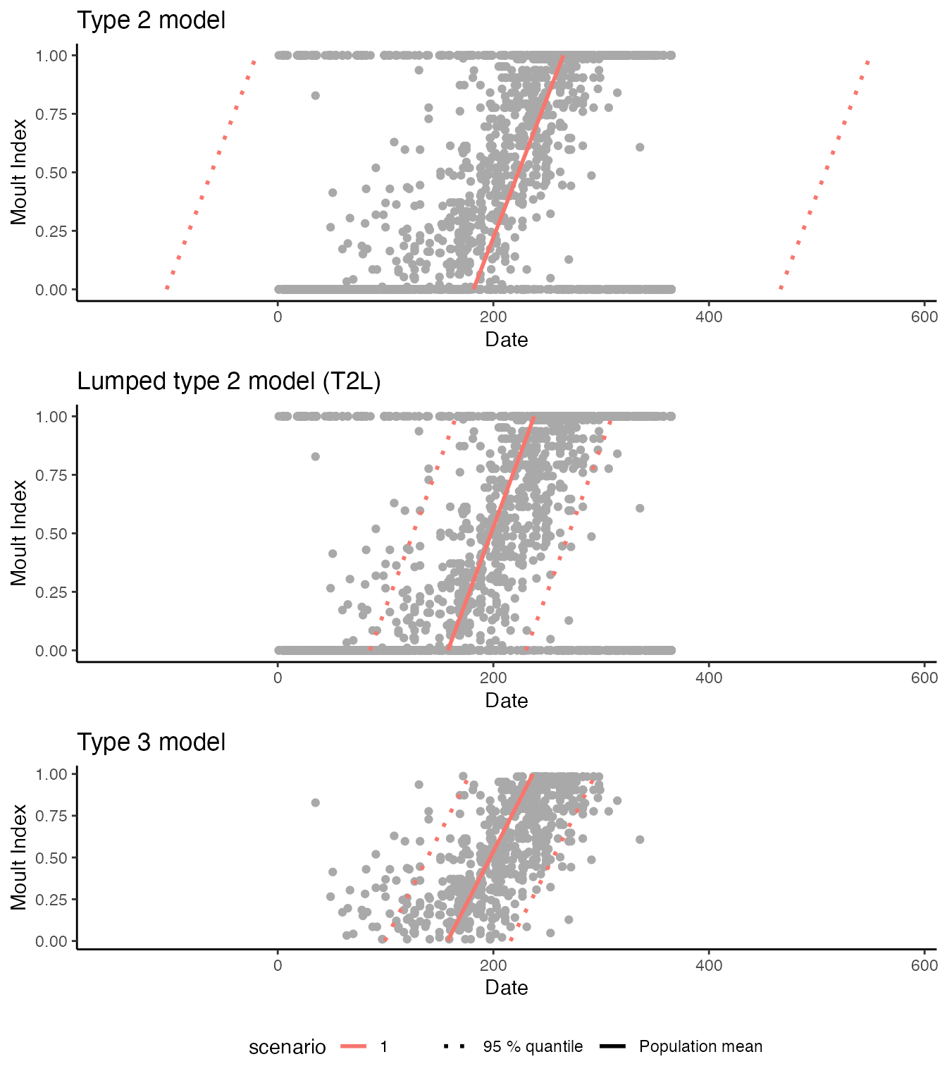
The moult plots make it clear that the standard type 2 model estimates an unrealistically large standard deviation of the start date, implying that the moult period for the population exceeds a calendar year. In contrast both the lumped type 2 model and the type 3 model give plausible estimates, in that both sets of estimates are consistent with published moult parameters for this species (Oschadleus 2005). However, the lumped type 2 model offers much higher nominal precision, as apparent from the model comparison plot.
compare_plot(mc3,mc2,mc2l) + theme(axis.text.x = element_text(angle = 30, vjust = 1, hjust=1))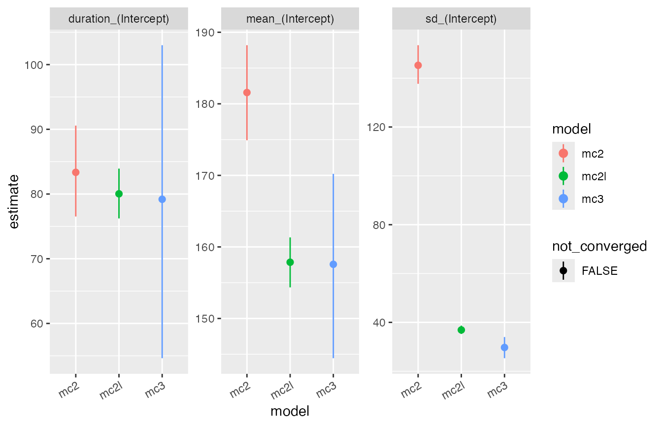
Repeated measures moult models
When the assumption of even sampling among and within moult categories is violated, the standard moult model can converge at biologically non-sensible results.
This problem can be greatly reduced when information about the pace of moult from within-season recaptures of individuals is explicitly incorporated into to the parameter estimation using the model.
The repeated measures model is currently implemented for data types
2, 3 and 5 in the moultmcmc function. The repeated measures
model is selected by supplying the optional argument
id_column which designates within season
recaptures, typically formed of a combination of ring number and
season.
We demonstrate this here using simulated data which is biased towards records of birds in the early stages of moult, based on a citizen science dataset of moult scores from Eurasian Siskins (Spinus spinus) (Insley, Beck, and Boersch-Supan (in prep)).
![Frequency distribution of moult records with respect to moult progress for actively moulting Eurasian Siskins [@insley2022moult] sampled in a sub-urban garden in Scotland (left) and seasonal progression of observed moult scores from the same dataset (right). Lines connect repeated observations of the same individuals.](extended-moult-models_files/figure-html/siskin-hist-1.png)
Frequency distribution of moult records with respect to moult progress for actively moulting Eurasian Siskins (Insley, Beck, and Boersch-Supan in prep) sampled in a sub-urban garden in Scotland (left) and seasonal progression of observed moult scores from the same dataset (right). Lines connect repeated observations of the same individuals.
The standard models are fitted by not specifying the
id_column input argument (which implies
id_column = NULL):
and the repeated measures models by passing the information about
bird identities to the moultmcmc() function:
#fit the equivalent recapture models
uz3_recap <- moultmcmc(moult_column = 'pfmg',
                       date_column = 'yday',
                       id_column = 'hexid',
                       start_formula = ~1,
                       duration_formula = ~1,
                       type = 3,
                       log_lik = FALSE,
                       data=siskins,
                       iter = 1000,
                       chain = 2,
                       cores = 2)
max(rowSums(get_elapsed_time(uz3_recap$stanfit)))
#
uz5_recap <- moultmcmc('pfmg',
                       'yday',
                       'hexid',
                       start_formula = ~1,
                       duration_formula = ~1,
                       type = 5,
                       log_lik = FALSE,
                       data=siskins,
                       iter = 1000,
                       chain = 2,
                       cores = 2)
#>             36.165 seconds (Total)
#> Chain 1:
#> Chain 2: Iteration: 1000 / 1000 [100%]  (Sampling)
#> Chain 2:
#> Chain 2:  Elapsed Time: 16.753 seconds (Warm-up)
#> Chain 2:                20.379 seconds (Sampling)
#> Chain 2:                37.132 seconds (Total)
#> Chain 2:
max(rowSums(get_elapsed_time(uz5_recap$stanfit)))
When comparing the results visually it is apparent that the moult period for the population predicted by the standard Type 3 models fails to encapsulate a substantial proportion of the observed data, whereas this is not the case for the repeated measures model. The bias in Type 5 model estimates is less severe.
#> Warning: Removed 1 row containing missing values or values outside the scale range
#> (`geom_point()`).
#> Removed 1 row containing missing values or values outside the scale range
#> (`geom_point()`).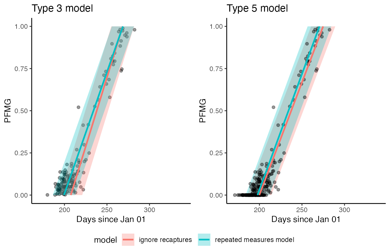
Standard type 3 and 5 moult models fitted to the Siskin dataset without considering within-season recaptures converge at biased parameter estimates (red lines and polygons). When recapture information is included in the model, the resulting fits (green lines and polygons) better encapsulate the observed data.
compare_plot(uz3,uz3_recap,uz5,uz5_recap) + theme(axis.text.x = element_text(angle = 30, vjust = 1, hjust=1), legend.position = 'bottom')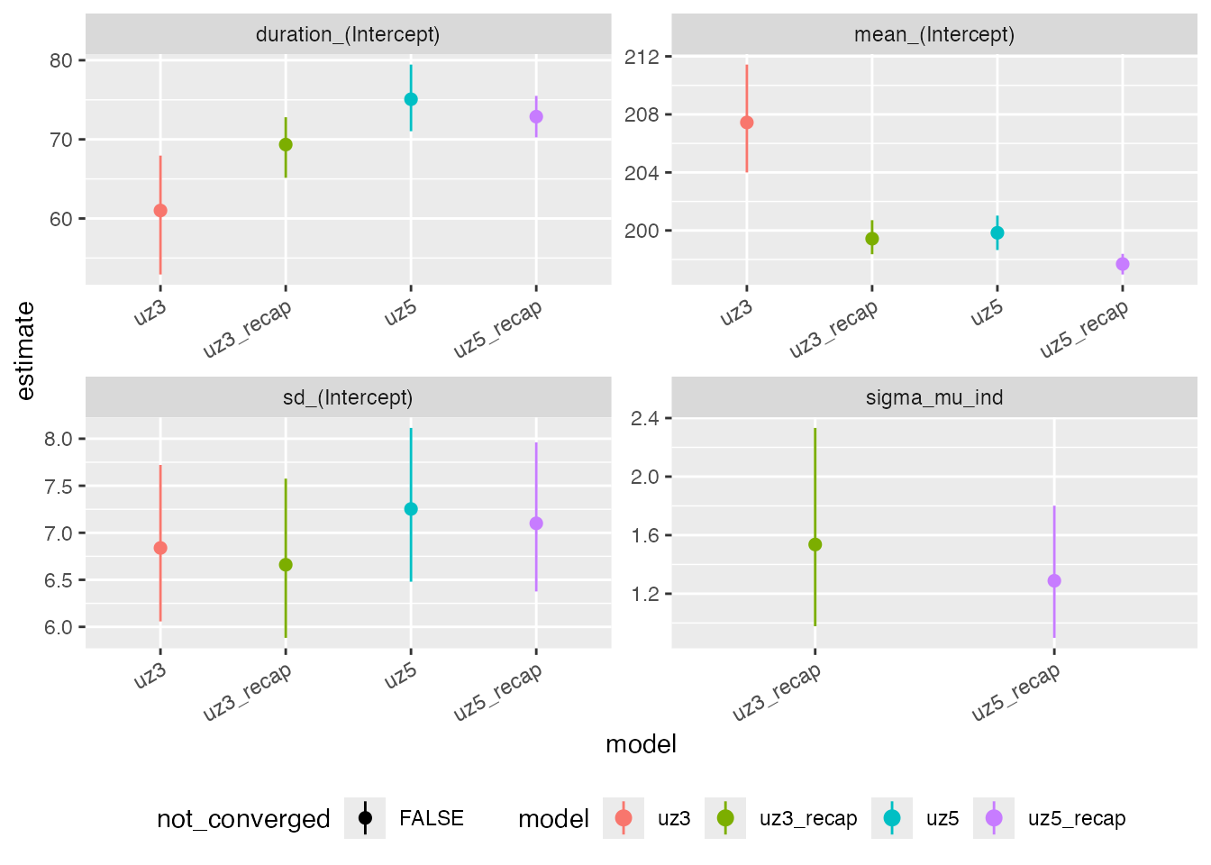
As these are simulated data we can also assess how well the recapture
model estimates individual start dates, by extracting the random
intercept estimates with the ranef() method and comparing
them to the simulated data.
ints <- ranef(uz3_recap) %>%
  as_tibble(rownames = 'hexid') %>%
  left_join(siskins) %>%
  group_by(id) %>%
  summarise(est_start = unique(mean),
            lci_start = unique(`2.5%`),
            uci_start = unique(`97.5%`),
            true_start = unique(start_date),
            true_dur = unique(duration),
            n_total = n(),
            n_active = sum(pfmg != 0))
#> Joining with `by = join_by(hexid)`

t3r_intercepts <- ggplot(ints,
                         aes(x = true_start - 196.83,
                             y = est_start,
                             ymin = lci_start,
                             ymax = uci_start,
                             fill = true_dur - 77.8)) +
  geom_pointrange(pch = 21) +
  scale_fill_gradient2() +
  theme_classic() +
  stat_smooth(method = 'lm') +
  ggtitle('T3R') +
  geom_abline(intercept = 0, slope = 1, lwd = 1, lty =2) +
  ylab('estimated start date') +
  xlab('true start date')

confint(lm(est_start ~ I(true_start - 196.83), data = ints))
#>                             2.5 %   97.5 %
#> (Intercept)            -3.6846662 1.245965
#> I(true_start - 196.83)  0.7649178 1.713936

ints <- ranef(uz5_recap) %>%
  as_tibble(rownames = 'hexid') %>%
  left_join(siskins) %>%
  group_by(id) %>%
  summarise(est_start = unique(mean),
            lci_start = unique(`2.5%`),
            uci_start = unique(`97.5%`),
            true_start = unique(start_date),
            true_dur = unique(duration),
            n_total = n(),
            n_active = sum(pfmg != 0))
#> Joining with `by = join_by(hexid)`

t5r_intercepts <- ggplot(ints,
                         aes(x = true_start - 196.83,
                             y = est_start,
                             ymin = lci_start,
                             ymax = uci_start,
                             fill = true_dur - 77.8)) +
  geom_pointrange(pch = 21) +
  scale_fill_gradient2() +
  theme_classic() +
  stat_smooth(method = 'lm') +
  ggtitle('T5R') +
  geom_abline(intercept = 0, slope = 1, lwd = 1, lty =2) +
  ylab('estimated start date') +
  xlab('true start date')

confint(lm(est_start ~ I(true_start - 196.83), data = ints))
#>                             2.5 %    97.5 %
#> (Intercept)            -0.3496927 0.9173969
#> I(true_start - 196.83)  0.8685707 1.0483337

cowplot::plot_grid(t3r_intercepts + theme(legend.position = 'none'),
                   t5r_intercepts + theme(legend.position = 'none'))
#> `geom_smooth()` using formula = 'y ~ x'
#> Warning: The following aesthetics were dropped during statistical transformation: fill.
#> ℹ This can happen when ggplot fails to infer the correct grouping structure in
#>   the data.
#> ℹ Did you forget to specify a `group` aesthetic or to convert a numerical
#>   variable into a factor?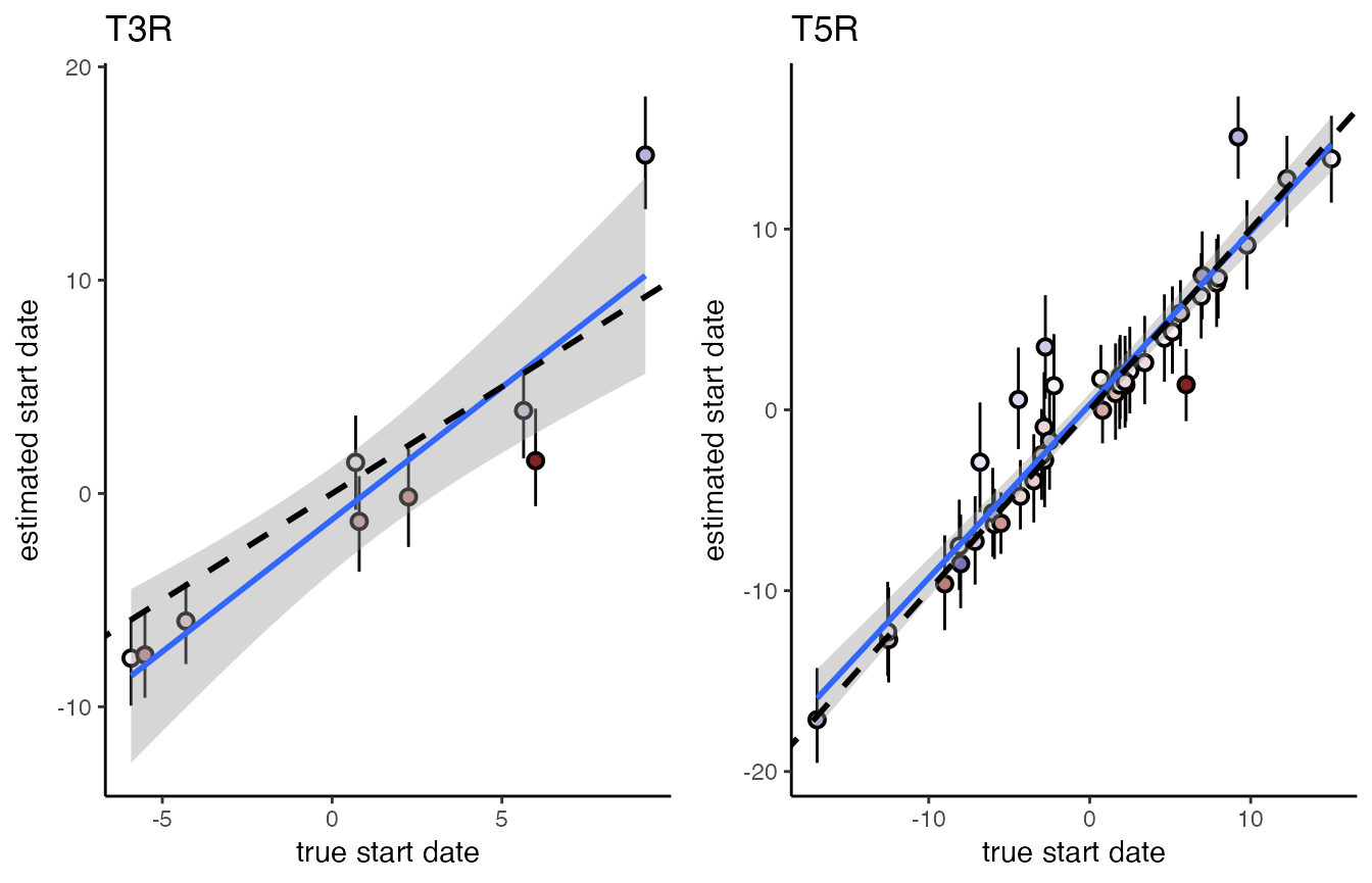
We find that agreement between simulations and estimates is good, even though the model does not explicitly account for heterogeneity in individual moult durations. For both models a regression of estimated versus true start dates has an intercept indistinguishable form 0 and a slope indistinguishable from 1.
Mixed moult records
moultmcmc also allows to fit a mixture of categorical
and continuous moult records, by combining the relevant likelihoods from
the type 1 and type 2 models, as originally suggested in Underhill and Zucchini (1988). This, so-called
Type 12 model can be employed to boost sample sizes
and/or allow better balancing of moult and non-moult records (Bonnevie 2010) when multiple types of records
are available.
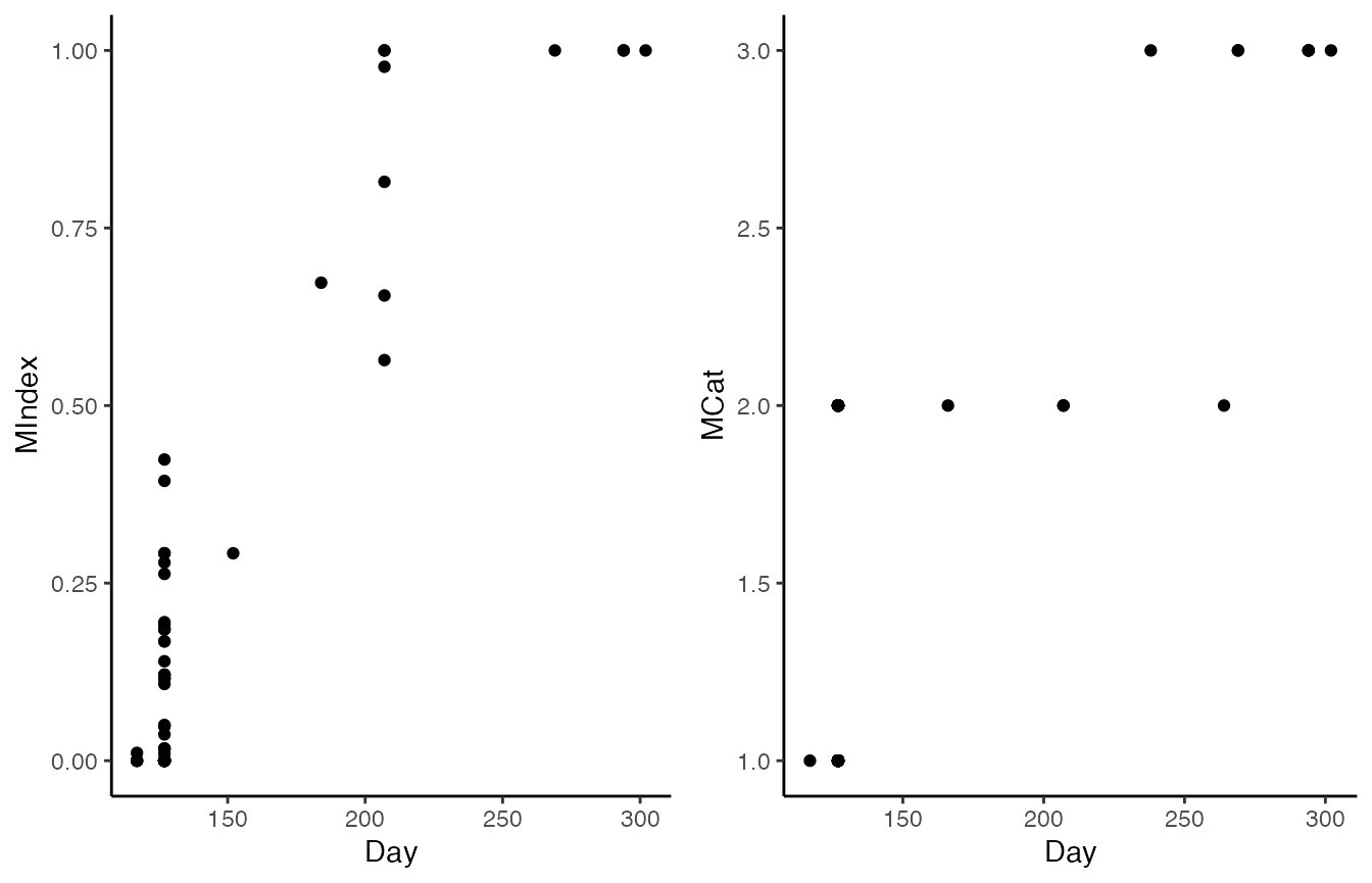
We can simulate such a dataset by splitting the
sanderlings dataset into two, and degrading the moult
scores in one subsample to moult categories
sanderlings <- moult::sanderlings

sanderlings$MCat[sanderlings$MIndex == 0] <- 1
sanderlings$MCat[sanderlings$MIndex == 1] <- 3
sanderlings$MCat[is.na(sanderlings$MCat)] <- 2
#introduce a couple of NAs
set.seed(1234)
sanderlings$keep_score <- sample(c(0,1), size = nrow(sanderlings), replace = TRUE)
sanderlings_scores <- subset(sanderlings, keep_score==1)
sanderlings_cat <- subset(sanderlings, keep_score==0)
sanderlings_cat$MCat[sanderlings_cat$MIndex == 0] <- 1
sanderlings_cat$MCat[sanderlings_cat$MIndex == 1] <- 3
sanderlings_cat$MCat[sanderlings_cat$MIndex != 1 & sanderlings_cat$MIndex != 0] <- 2
sanderlings_cat$MIndex <- NULL

cowplot::plot_grid(
  ggplot(sanderlings_scores, aes(x = Day, y = MIndex)) + geom_point() + theme_classic(),
  ggplot(sanderlings_cat, aes(x = Day, y = MCat)) + geom_point() + theme_classic()
)
The two datasets can then be pieced together again, and the function
consolidate_moult_records is used to consolidate and recode
moult score and moult category data.
sanderlings_combined <- bind_rows(sanderlings_scores, sanderlings_cat)
sanderlings_combined$MIndexCat <- consolidate_moult_records(sanderlings_combined$MIndex, sanderlings_combined$MCat)
We can then fit Type 1 and Type 2 models to each of the split datasets, as well as the Type 12 model for the recombined dataset, and for reference a Type 2 model to the original data.
fit_scores <- moultmcmc(moult_column = "MIndex",
                 date_column = "Day",
                 data = sanderlings_scores,
                 type = 2,
                 log_lik = FALSE,
                 chains = 1)

fit_cat <- moultmcmc(moult_column = "MCat",
                 date_column = "Day",
                 data = sanderlings_cat,
                 type = 1,
                 log_lik = FALSE,
                 chains = 1)

fit_combined = moultmcmc(moult_column = "MIndexCat",
                 date_column = "Day",
                 data = sanderlings_combined,
                 type = 12,
                 log_lik = FALSE,
                 chains = 1)

fit_original = moultmcmc(moult_column = "MIndex",
                 date_column = "Day",
                 data = sanderlings,
                 type = 2,
                 log_lik = FALSE,
                 chains = 1)
compare_plot(fit_scores, fit_cat, fit_combined, fit_original) + theme(axis.text.x = element_text(angle = 30, vjust = 1, hjust=1))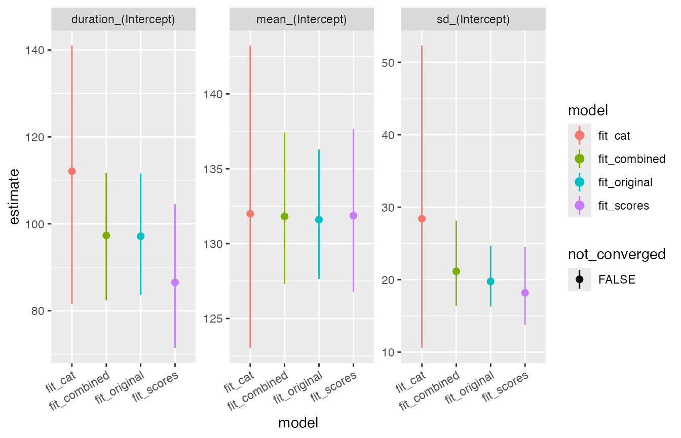 The estimates from the combined model (T12) are closer to the estimates
from the original dataset, than estimates from either partial
dataset.
The estimates from the combined model (T12) are closer to the estimates
from the original dataset, than estimates from either partial
dataset.