04 Nov 2019
Philipp Boersch-Supan
paper
Tweet this!
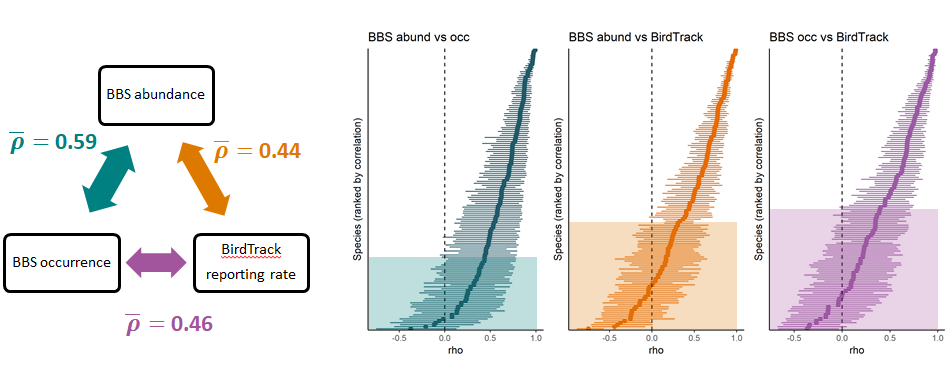
A new paper on bird population trend models 🐦📈 led by myself in collaboration with Amanda Trask and Stephen Baillie has appeared in Biological Conservation: Robustness of simple avian population trend models for semi-structured citizen science data is species-dependent
We compared & myself compared population trends derived from structured breeding bird surveys and unstructured bird lists from the BirdTrack citizen science scheme using a simple statistical model, i.e. one that did not explicitly account for preferential sampling in the latter dataset. We found that - even when not accounting for sampling bias - reporting rate trends from BirdTrack broadly resembled those derived from the structured survey for common and widespread birds. However, this agreement was less good for rare species and those with little or uncertain population change.
You can read a full summary of the paper at the BTO website.
A free preprint of the paper is available at this link.
30 Oct 2019
Philipp Boersch-Supan
paper
Tweet this!
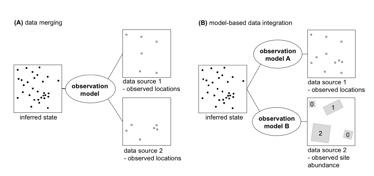
A new paper led by Nick Isaac and Bob O’Hara on data integration approaches for biodiversity records has just been published in Trends in Ecology and Evolution: Data Integration for Large-Scale Models of Species Distributions.
This review article highlights novel analysis approaches, conceptually based on point-process models, to better understand species distributions by integrating data from a wide variety of surveys and other citizen science projects.
03 Jan 2019
Philipp Boersch-Supan
paper Bayes R Software
Tweet this!
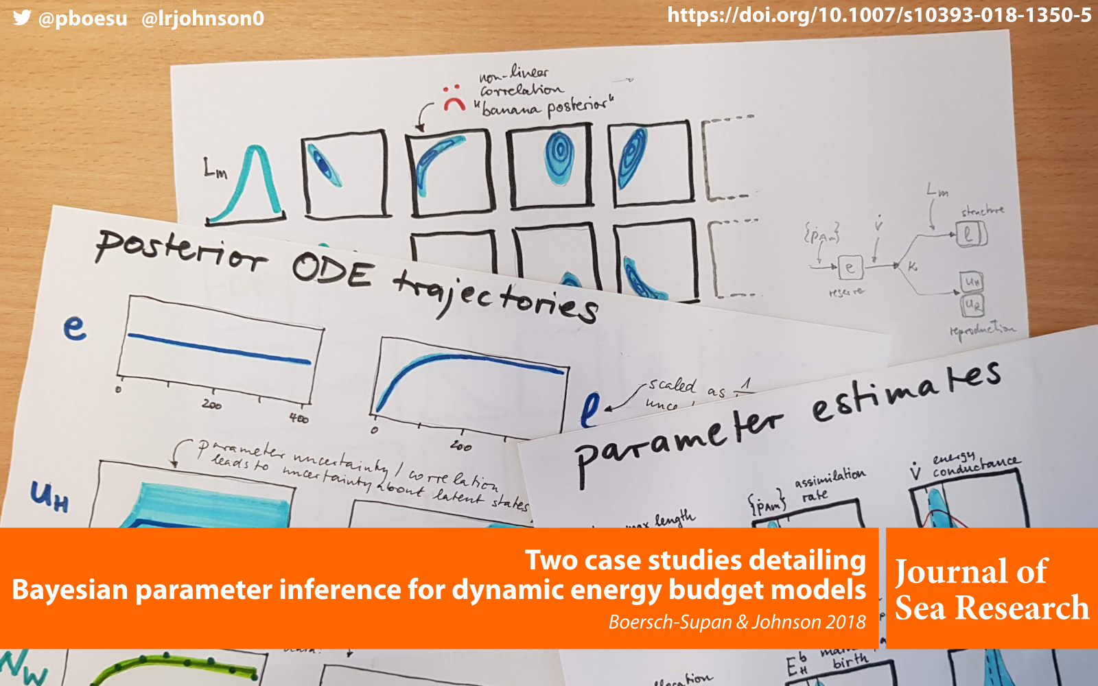
A new paper with Leah Johnson on Bayesian inference in Dynamic Energy Budget models has just been published in the Journal of Sea Research: Two case studies detailing Bayesian parameter inference for dynamic energy budget models.
Our paper walks through two case studies to illustrate how the parameters for two different types of dynamic energy budget models can be inferred from data using the deBInfer R package.
An open access preprint can be found on bioRxiv and the code underlying the paper is archived on zenodo.
09 Aug 2018
Philipp Boersch-Supan
paper disease ecology
Tweet this!
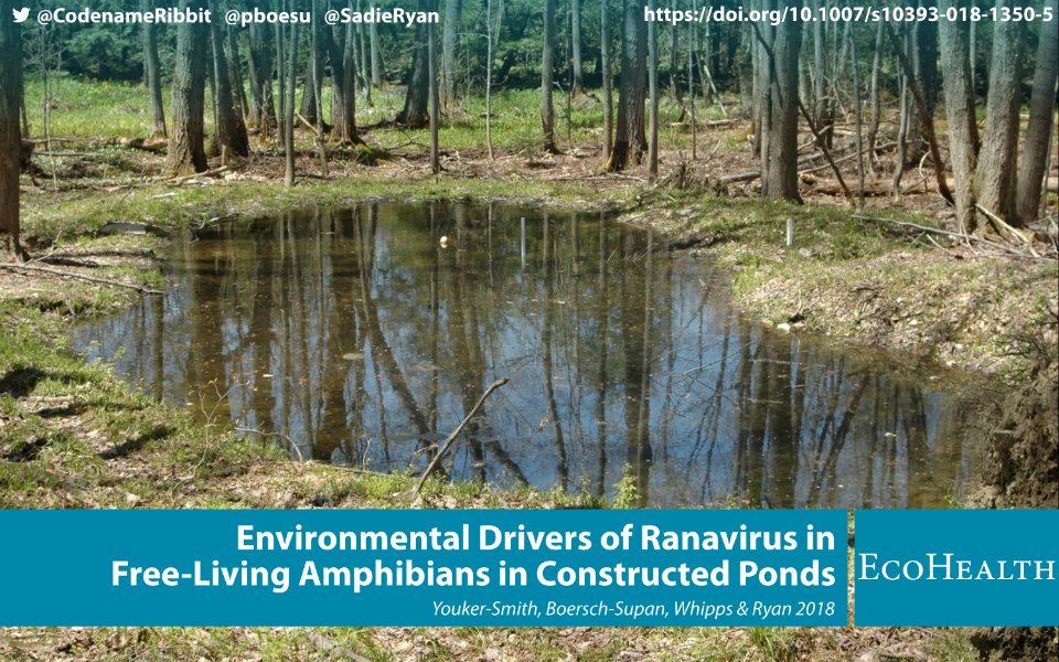
A new paper with the QDEC Lab and collaborators from SUNY-ESF on the prevalence of ranavirus in tadpoles of free-living frogs has just been published in EcoHealth: Environmental Drivers of Ranavirus in Free-Living Amphibians in Constructed Ponds.
Our paper uses generalised linear models fitted in a Bayesian inference framework to analyze four years of Frog virus 3 prevalence and associated environmental parameters in populations of wood frogs (Lithobates sylvaticus) and green frogs (Lithobates clamitans) in a constructed pond system. We identified important variables to measure in assessments of ranaviral infection risk in newly constructed ponds, including effects of zooplankton, which have not been previously quantified in natural settings. High prevalence was best predicted by low temperature, high host density, low zooplankton concentrations, and Gosner stages approaching metamorphosis.
17 Feb 2018
Philipp Boersch-Supan
rstats
Tweet this!
Yesterday I came across Gordon Pennycook’s tweet about moving in academia:
So given that there’s a transatlantic move coming up for me to take up my first permanent research position at the British Trust for Ornithology, I thought, why not figure this out quickly using R.
library(ggmap)# for geocoding and plotting
library(geosphere)# for distance calculations
library(knitr)# for making a nice table
I used ggmap::geocode to look up the coordinates of each station on my academic career path:
academic_places <- geocode(c(home = "Neustadt an der Weinstrasse",
                             undergrad = "Marburg an der Lahn",
                             masters_phd = "St Andrews, Fife",
                             phd = "Oxford, Oxfordshire",
                             postdoc1 = "Cambridge, UK",
                             postdoc2a = "Tampa, FL",
                             postdoc2b = "Gainesville, FL",
                             job = "Thetford"),
                           source = "dsk")
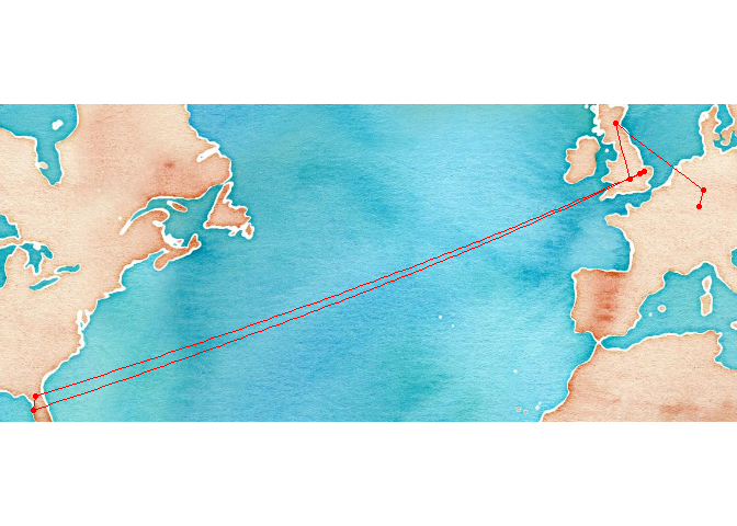
A quick plot to sanity check the locations
#make a map
qmplot(lon, lat, data = academic_places, maptype = "watercolor", color = I("red")) + geom_path(color = "red")
I then used the geosphere package to calculate sequential distance between stations
#calculate distances
distances_m <- distGeo(as.matrix(academic_places[,2:3]))

#transform units
distances_km <- distances_m/1000
distances_mi <- distances_m/1609
And lastly, I made a table to sum up everything.
#make a table
kable(data.frame(stage = c(academic_places[-1,1], "Total"),
                 distance_km = round(c(distances_km, sum(distances_km))),
                 distance_mi = round(c(distances_mi, sum(distances_mi)))))
| stage |
distance_km |
distance_mi |
| undergrad |
172 |
107 |
| masters_phd |
992 |
617 |
| phd |
516 |
321 |
| postdoc1 |
107 |
67 |
| postdoc2a |
7121 |
4426 |
| postdoc2b |
185 |
115 |
| job |
7005 |
4354 |
| Total |
16099 |
10006 |